In this post, we present a visual approach for exploring genotypic data and performing genome-wide association and epistasis analysis using a simulated phenotype for the YRI (Yoruba in Ibadan, Nigeria) cohort from the International HapMap project. We start first with quality control process for SNPs and samples.
1. Quality Control
Data for genome-wide association and epistasis analysis demand a fair amount of pre-processing and quality control; various quality metrics are commonly used to filter out data of low quality and data that bias or alter the accuracy of the analysis. This pre-analytical quality control phase is a three-step process that we can summarize them as follow: (1) generating descriptive statistics from SNPs and samples (2) defining quality thresholds (3) eliminating SNPs and samples that don’t meet the quality thresholds.
1.1. SNP Call Rate
The SNP call rate is calculated per SNP and defined as the proportion of samples for which the corresponding SNP information is available and measured with adequate accuracy. SNPs with very low call rate decrease the accuracy of the analysis and unnecessarily increase type-1 error and should be filtered out.
PLINK –missing command produces excellent variant-based and sample-based missing data reports that we can utilize. We used R ggpubr library to visualize the SNP call rate distribution. Figure 1. shows SNP call rates with adequate quality; all SNPs have call rate above 90% and only 19636 SNPS (1.38%) have call rate below 98%. Based on this graph as a visual guide, we decided to filter out SNPs with call rate below 98% using PLINK –geno command.

1.2. SNP Minor Allele Frequency
Minor allele frequency (MAF) is the frequency of the second, less common, allele at a biallelic genomic site. The allele frequency spectrum in genome-wide biallelic variants has diversified nature; some variants show only one allele across all samples (monomorphic), other variants show two different alleles (polymorphic) with one allele showing up at a very low frequency (rare allele). The association between a variable phenotype and a rare allele might exist in very few individuals; hence, no sufficient power to detect this type of association. In order to avoid this problem, we apply SNP-level filtering based on MAF and exclude SNPs with very low MAF.
PLINK –freq command produces a minor allele frequency report. Figure 2. shows the distribution of SNP MAF ; based on the graph, we decided to exclude 117159 (8.32%) SNPs with MAF less than 1%.

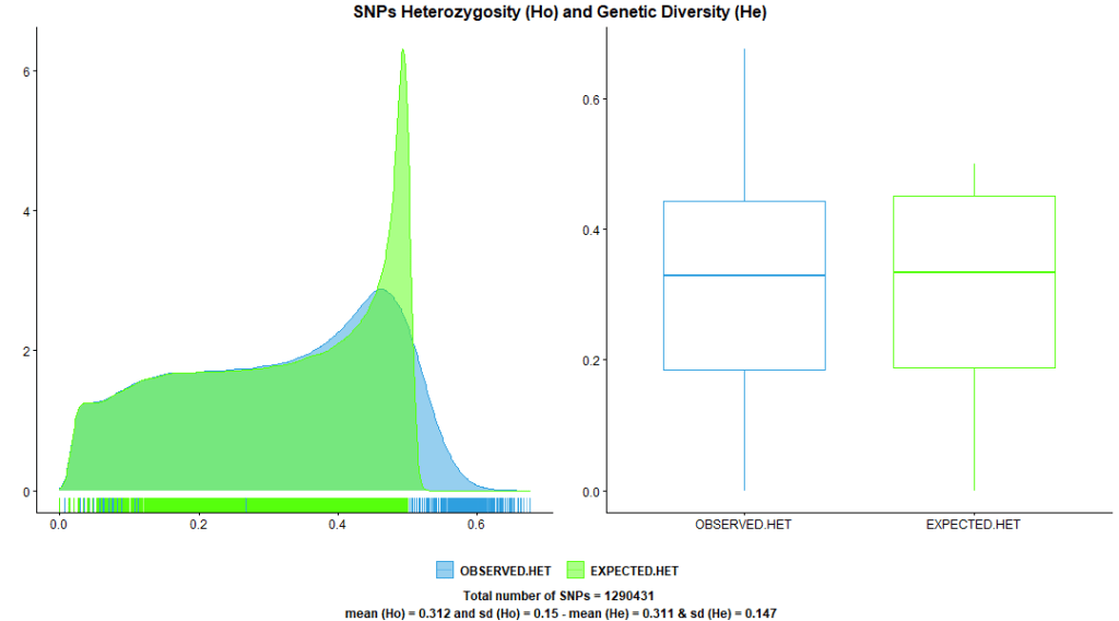
1.3. SNP Heterozygosity and Genetic Diversity
Heterozygosity is the proportion of heterozygotes per SNP in relation to all genotypes. This quality metric compares actual SNP heterozygosity to its expected heterozygosity (also called genetic diversity).
PLINK –hardy command produces both of these statistics, SNPs expected and observed heterozygosity. Figure 3. shows approximately equal heterozygosity and genetic diversity statistics after applying the previous quality control steps, an indicator that we are heading in the right direction.
1.4. Sample Call Rate
The sample call rate is calculated per sample and defined as the proportion of samples for which the corresponding SNP information is available and measured with adequate accuracy. Sample filtering based on call rate is used to exclude samples with poor DNA quality.
PLINK –missing command produces sample-based missing data report. Figure 4. shows sample call rates with adequate quality; all samples have call rate above 98% so we didn’t exclude any samples.

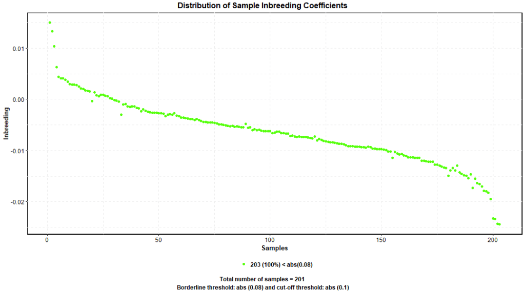
1.5. Inbreeding
Inbreeding is the production of offsprings from breeding of individuals that are closely related genetically. Inbreeding results in increased homozygosity, also called fixation, which in turn increases the chances of offsprings being affected by recessive traits.
Probability theory is utilized to assess inbreeding; the inbreeding coefficient (F), also called fixation index, is the probability that both alleles in one genomic locus are identical and derived from the same ancestral allele – identical by decent (IBD). Excessive inbreeding leads to a decreased biological fitness of the affected population; genome wide association analysis assumes a population with normal biological fitness; therefore, it’s highly desirable to exclude samples with inbreeding coefficient less than -0.1 or greater than 0.1. Generally, the average inbreeding coefficient for all the samples should be around zero.
PLINK –het command produces F coefficient estimates. Figure 5. shows F distribution around 0 and all the samples have F coefficient below 0.1. Therefore, we didn’t exclude any samples based on this quality threshold.
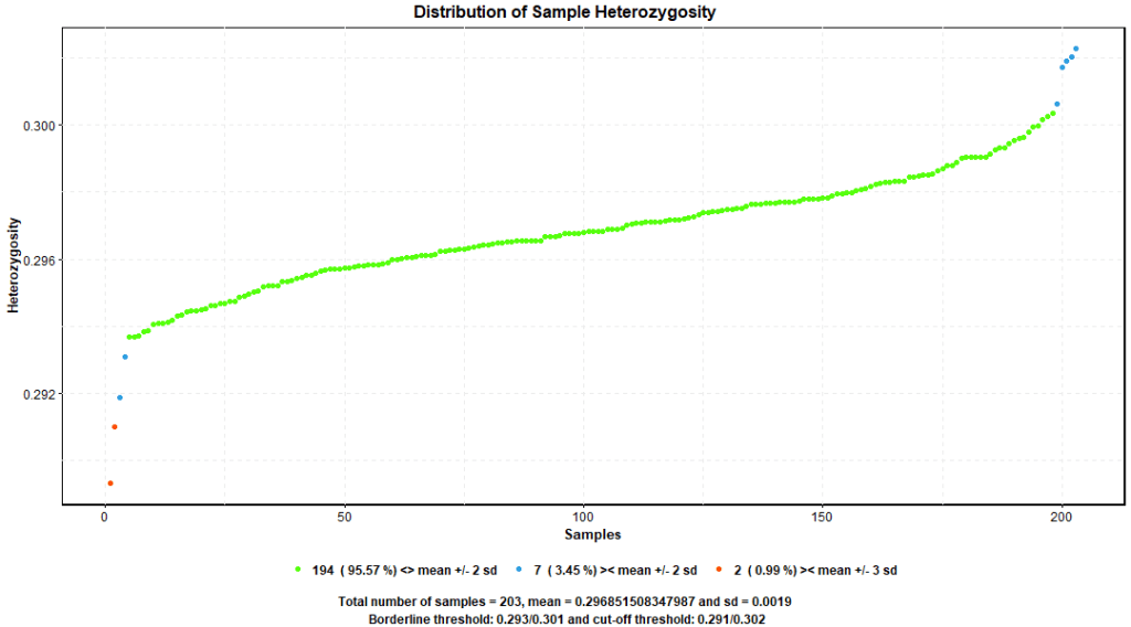
1.6. Sample Heterozygosity
Heterozygosity is the proportion of heterozygote genotypes in relation to all genotypes, it is a common practice to evaluate heterozygosity on samples. Essentially, if a sample’s heterozygosity is high, it can be an indicator of DNA contamination or a sign of true deviation of that sample from the bulk of data samples. Removal of samples that depart 3 standard deviations (+/- 3SD) from the mean is a reasonable approach to ensure sample consistency.
PLINK –hardy command produces statistics about observed and expected number of homozygotes, given these statistics, we can produce a distribution of sample heterozygosity. Figure 6. shows 2 samples depart more than -3SD from the mean. We excluded these 2 samples using PLINK –remove command.
1.7. Relatedness Estimate
Relatedness, also called the coefficient of relationship, is the measure of the degree of consanguinity between two individuals. Relatedness analysis could be used to identify replicates and highly related samples. On the contrary, it could be used to identify samples that show true divergence as a result of poor DNA quality.
The concept of identity by decent (IBD) is utilized to asses relatedness; a pair-wise sample relatedness measure (Pi Hat) is defined as: Pi Hat = P(IBD=2) + 0.5*P(IBD=1).
PLINK –genome produces IBD and IBS statistics. Figure 7. shows 57 samples having 114 have high relatedness Pi Hat values. Conservative researchers may choose to exclude these samples, if this doesn’t significantly affect their study.

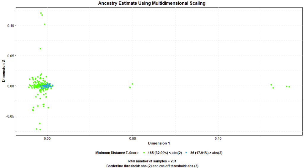
1.8. Ancestry Estimate
Ancestry is the study of a given population structure, it refers to genetic differences that exist between individuals from different families, groups, or geographical regions. Ancestry could be estimated and understood using multidimensional scaling (MDS) and calculation of nearest neighbor distances between samples.
PLINK –mds-plot command produces multidimensional scaling report and –neighbor command nearest neighbor distance report containing per sample Z score calculated as an estimate of IBS nearest distance with neighboring samples. We considered samples that depart 6 standard deviations (+/- 6SD) from the mean Z score as outliers. Figure 8. shows few samples departed more than 2 SD from the mean but no samples exceeded the +/- 6 SD threshold.
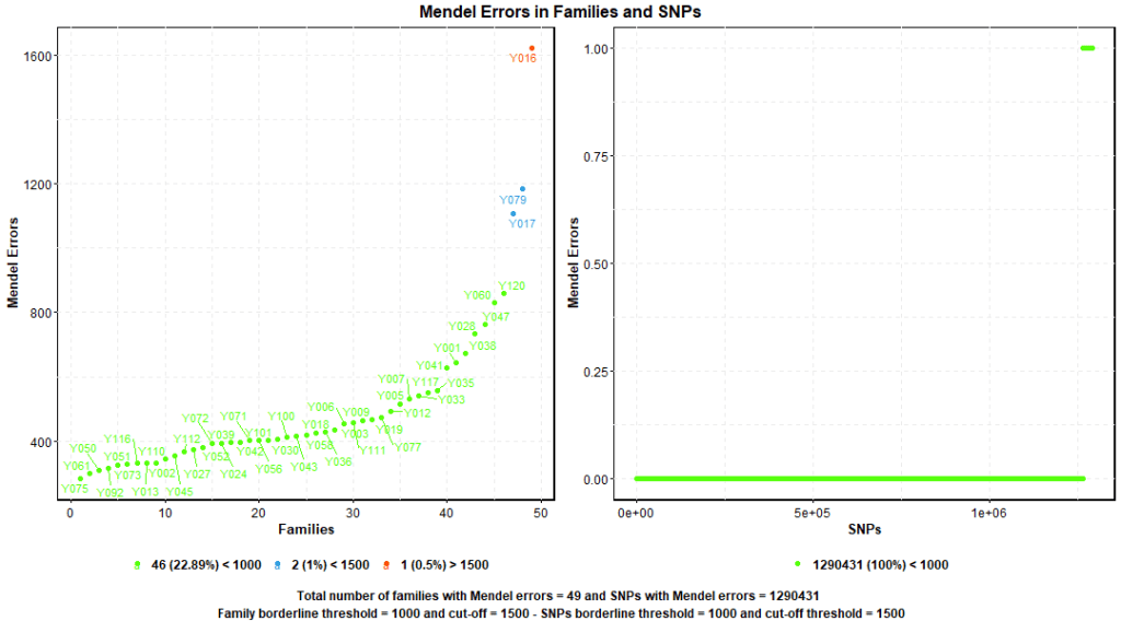
1.9. Mendel Errors
Mendel errors counts alleles in individual samples that don’t conform to the principles of Mendelian inheritance. This test requires accurate family/trio data. A small number of Mendel errors exists within each family, however, when the number exceeds a certain threshold, this indicates a genotyping error or inaccurate family data.
PLINK –mendel command scans the dataset for Mendel errors in families and SNPs. Figure 9. shows one of the families has about 1600 Mendel errors which is still acceptable. Some conservative researchers may consider revising the data or exclude this family from the analysis.
1.10. Hardy-Weinberg Equilibrium
Hardy–Weinberg equilibrium (HWE) principle describes the relationship between genotypic frequencies and allelic frequencies in a population and how they should stay in equilibrium (theoretically) across generations. HWE principle is valid under few assumptions that include: an infinite size population and independent random mating. Obviously real populations do not adhere to these assumptions but we can benefit from knowing how far a population has deviated from HWE theoretical principle.
Statistically, we assume HWE principle as the distribution null hypothesis of a genotypic variant; when a genotypic variant is statistically different from the model’s null assumption, this indicates a genotyping error or a biologically relevant factor acting on the population. In case of disease phenotypes, it’s highly advisable to include genotypic variants that violate HWE principal as they could be the disease-causing variants.
PLINK –hardy command generates p-values as an output of equilibrium exact test measuring the deviation from the distribution null hypothesis. We use p-value cut-off threshold of 1e-06. Figure 10. shows no SNPs deviated significantly from the null hypothesis.

2. Genome Wide Association Analysis
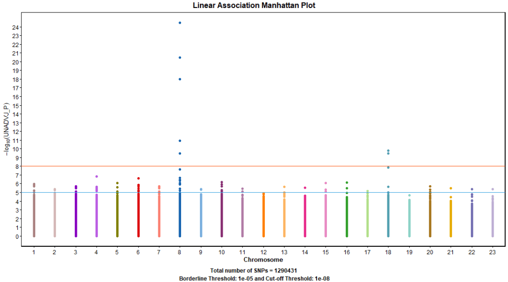
2.1. Single Marker Analysis
The first standard approach to GWAA is single marker tests of SNPs. This approach involves understanding and preparing the phenotype then regressing each SNP separately on the given trait, while adjusting for clinical, environmental, and demographic factors.
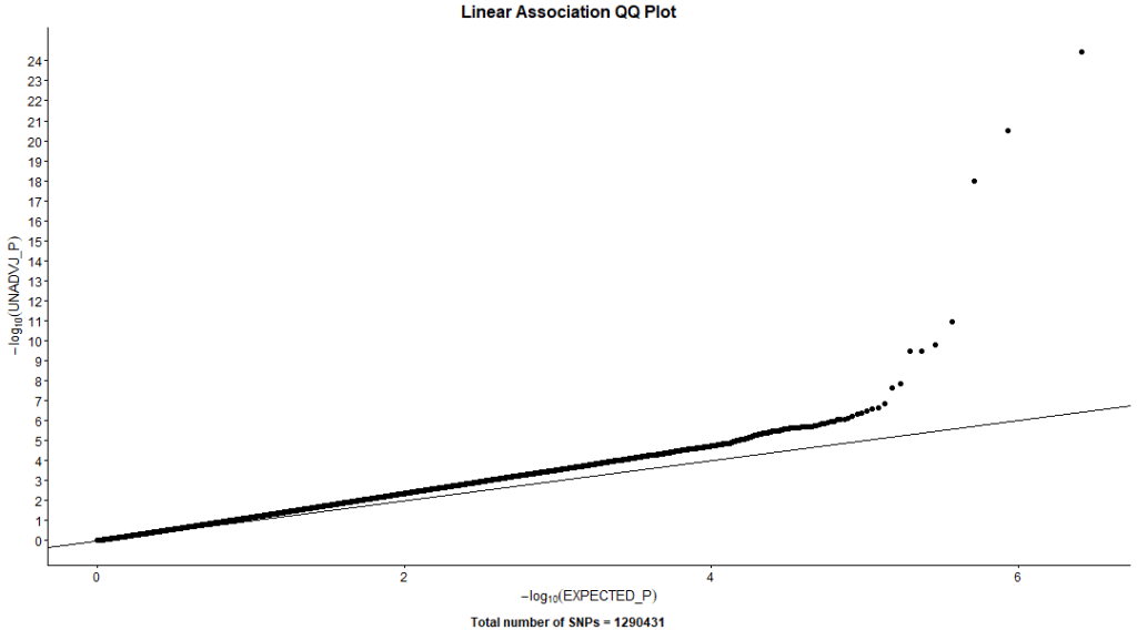
PLINK –linear command used linear models to test the association with our simulated phenotype. Figure 11. shows 2 signals; one on chromosome 8 (5 SNPs) and the other on chromosome 18 (2 SNPs). Table 1. shows more detailed information about significant SNPs and their closest genes.
| ID | UNADJ | FDR_BY | Chromosome | Position | Gene | SNP Gene Hit |
| rs1494272 | 3.60E-25 | 6.81E-18 | 8 | 104194973 | BAALC | Overlapping |
| rs713368 | 3.32E-21 | 3.13E-14 | 8 | 104196713 | BAALC | Overlapping |
| rs7817115 | 1.00E-18 | 6.33E-12 | 8 | 104194150 | BAALC | Overlapping |
| rs4645535 | 1.18E-11 | 5.56E-05 | 8 | 104196509 | BAALC | Overlapping |
| rs9653004 | 1.69E-10 | 0.000638 | 18 | 35537135 | MIR4318 | Following |
| rs1497456 | 3.41E-10 | 0.000921 | 8 | 104181000 | BAALC | Overlapping |
| rs11664246 | 3.41E-10 | 0.000921 | 18 | 35535315 | MIR4318 | Following |
| rs7240706 | 1.36E-08 | 0.03211 | 18 | 35527130 | MIR4318 | Following |
| rs1391118 | 2.25E-08 | 0.04722 | 8 | 104155852 | BAALC | Overlapping |
| rs2030001 | 1.41E-07 | 0.2655 | 4 | 68257391 | CENPC | Preceding |
| rs3736042 | 2.19E-07 | 0.3756 | 8 | 104146731 | BAALC-AS2 | Overlapping |
| rs1408482 | 2.51E-07 | 0.3956 | 6 | 7524604 | DSP | Preceding |
| rs1000461 | 3.40E-07 | 0.4945 | 8 | 104186211 | BAALC | Overlapping |
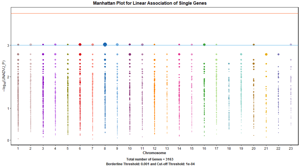
2.2. Single Gene Analysis
Based on the results of GWAA, various in-depth analyses could be performed. The single gene analysis uses longer DNA strand instead of single SNP as a unit of analysis. After overlapping significant SNPs to genes, we selected 3201 genes, each block has at least one SNP from the single marker tests with unadjusted p-value less than 0.01.
For each selected gene, we performed single marker tests for all SNPs then we selected a subset of significant SNPs in linkage equilibrium as a representative list for the gene, the average additive effect is set as an original association score. Empirical p-value is generated by iterating the previous steps 32768 times, the empirical p-value is estimated based on how often permutation-based gene association scores greater than or equal to the originally generated association score.
PLINK –linear command combined with –set-test command can be used to perform this analysis. Figure 13. shows a Manhattan plot for the results where the diameter of the points represents the number of significant SNPs within the boundaries of the associated gene. Table 2. shows that gene BAALC appears among the top list of genes which is consistent with the single marker analysis result. Other genes appeared such MAP3K5 and SAXO1 which worth further investigations. But remember that, this phenotype is simulated and doesn’t reflect a real trait.
| Gene | EMP_P_Value | Chromosome | Start Position | End Position | NSNP | NSIG |
| BAALC | 0.000976 | 8 | 104152921 | 104242533 | 45 | 31 |
| MAP3K5 | 0.000976 | 6 | 136878187 | 136977598 | 44 | 15 |
| SAXO1 | 0.000976 | 9 | 18927891 | 19033256 | 96 | 28 |
| LINC00320 | 0.001951 | 21 | 22114913 | 22175426 | 33 | 15 |
| VAV2 | 0.000976 | 9 | 136627016 | 136857446 | 140 | 31 |
| KCNK5 | 0.001951 | 6 | 39156747 | 39197251 | 33 | 14 |
| LHFPL3 | 0.000976 | 7 | 103969104 | 104549003 | 349 | 71 |
| PRIM2 | 0.000976 | 6 | 57182422 | 57191161 | 6 | 3 |
| OR2A5 | 0.000976 | 7 | 143747495 | 143748430 | 2 | 2 |
| NCAM1-AS1 | 0.000976 | 11 | 113140254 | 113144623 | 1 | 1 |
| ORM2 | 0.000976 | 9 | 117092069 | 117095536 | 1 | 1 |
| WDR54 | 0.000976 | 2 | 74648885 | 74652882 | 1 | 1 |
| MIR1256 | 0.001951 | 10 | 74119698 | 74336541 | 113 | 45 |
| GRIN2A | 0.000976 | 16 | 9847265 | 10276263 | 364 | 71 |
| SDK1 | 0.000976 | 7 | 3341080 | 4308631 | 550 | 103 |
| LINC-PINT | 0.000976 | 7 | 130628919 | 130791789 | 88 | 16 |
| NLRP1 | 0.002927 | 17 | 5404719 | 5487832 | 41 | 21 |
| STK32B | 0.000976 | 4 | 5053527 | 5502725 | 313 | 52 |
3. Genome Wide Interaction Analysis
Following the identification of genetic markers by whole genome wide association analysis, we performed further analysis focusing on the detection of effects due to significant genetic loci interaction with other genetic loci, also known as epistasis, these effects may not be identified by using single marker tests. Detecting interactions that provide valuable insights into relevant biological and biochemical pathways is one of the most practical aims of epistatic studies.
For a quantitative trait and two SNPs modelled using the additive genetic model, the test for a pair-wise interaction using linear regression model can be represented as follow:
y= x0 + x1 A + x2 B + x3 A.B + e
Where: y is the quantitative phenotype, A and B represent the allelic dosage for each SNP, and the test for interaction is based on the coefficient of the interaction term x3.
All pairwise combinations of SNPs can be tested but this is computationally very expensive. Therefore, we selected a list of 1883 SNPs in linkage equilibrium with genome wide significant p-value less than less than 0.01 , the input list is the same list of representative SNPs for genes used in the single gene association analysis.
PLINK –epistasis command can be used to perform this analysis. Table 3. shows pairs of SNPs that are significantly associated with our simulated phenotype and Figure 14. shows the pathway enriched using genes overlapping with the list of pairs of interacting SNPs to gain functional insights about these interactions. The functional enrichment was done using R clusterProfiler library.
| SNP_ID_1 | Chromosome | Position | Gene | SNP_Gene_Hit | SNP_ID_2 | Chromosome | Position | Gene | SNP_Gene_Hit | P_Value | FDR |
| rs4421580 | 1 | 15289210 | KAZN | Overlapping | rs10736312 | 10 | 124088367 | BTBD16 | Overlapping | 1.25E-08 | 1.38E-05 |
| rs9426910 | 1 | 170914071 | MROH9 | Overlapping | rs1181736 | 7 | 141130932 | TMEM178B | Overlapping | 7.00E-08 | 3.13E-05 |
| rs2744454 | 6 | 52955142 | FBXO9 | Overlapping | rs4764497 | 12 | 6428116 | PLEKHG6 | Overlapping | 1.52E-07 | 3.58E-05 |
| rs9859728 | 3 | 9736899 | MTMR14 | Overlapping | rs6538405 | 12 | 78234093 | NAV3 | Overlapping | 1.88E-07 | 3.58E-05 |
| rs4084164 | 11 | 62201458 | AHNAK | Overlapping | rs2046682 | 11 | 106678032 | GUCY1A2 | Overlapping | 2.85E-07 | 3.85E-05 |
| rs10214977 | 7 | 94727327 | PPP1R9A | Overlapping | rs7966000 | 12 | 3682483 | PRMT8 | Overlapping | 4.25E-07 | 4.62E-05 |
| rs2336646 | 1 | 12315671 | VPS13D | Overlapping | rs7640471 | 3 | 29462116 | RBMS3 | Overlapping | 4.74E-07 | 4.86E-05 |
| rs6984772 | 8 | 73817199 | KCNB2 | Overlapping | rs874564 | 10 | 78672265 | KCNMA1 | Overlapping | 5.14E-07 | 5.07E-05 |
| rs656489 | 2 | 75060099 | HK2 | Overlapping | rs604663 | 10 | 6504126 | PRKCQ | Overlapping | 5.61E-07 | 5.14E-05 |
| rs17068919 | 5 | 167085745 | TENM2 | Overlapping | rs11993800 | 8 | 27885843 | NUGGC | Overlapping | 6.72E-07 | 5.24E-05 |

